Time Scheduling Calculations
Time Scheduling Calculations
Suppose you are working in a project during some set time interval. For the interval, team members decide on a sum of predicted times (including all the tasks within such time interval) labeled as $S_{pt}$. Throughout the span of the time interval, team members continuously participate to keep track of time spent on each task. Then, at the end, they add all the times (they actually spent on each task) obtaining the sum of actual times labeled as $S_{at}$.
We obtain a ratio, say $\lambda$, where $\lambda = \cfrac{S_{at}}{S_{pt}}$. If the value of $\lambda < 1$ the team has managed to completed all the tasks earlier than predicted. On the other hand, if $\lambda > 1$, then the team has not managed to complete all the tasks as late as the predicted times (resulting in a project overdue).
We may calculate a value, say $d$, expressing the percentage by which $S_{at}$ deviates from $S_{pt}$. Hence: $d = | \lambda - 1 | \times 100$. E.g., if, in a certain project, $\lambda = 1.05$, then the additional project overdue is $5\%$.
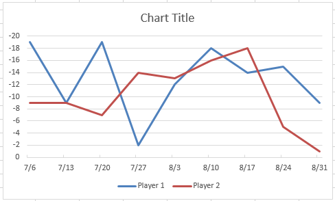
Moreover, the individual times can be represented as points in the Cartesian coordinate system via a point-to-point graph. Namely, we can have a two such graphs: one for the predicted time, the latter for the actual time.
A code snippet example taken from R (one point-to-point graph):
x  <- seq(1, 10, length.out = 10)        # x coordinates: 1 through 10
y1 <- c(1, 10, 5, 3, 4, 5, 6, 7, 8, 9)  # dummy y1 coordinates - red color (estimate)
y2 <- c(1, 3, 1, 4, 10, 9, 8, 7, 6, 4)  # dummy y2 coordinates - blue color (actual)

# estimated time + plot
plot(x, y1, col = "red", lwd = 2,
    type = "l", xlab = "week", ylab = "hour", main = "Point-to-point Graph")

lines(x, y2, col = "blue", lwd = 2) # actual time

legend("topright", legend = c("Estimate", "Actual"),
        col = c("red", "blue"), lwd = 2)
Out (example):